As the first phase of HEVC standard (single layer video coding standard) comes close to finalization, scalable extensions of HEVC have been under discussion since the 7th JCT-VC meeting. The final call for proposal (CfP) [1] was issued jointly by ITU-T/VCEG and ISO/IEC/MPEG in July 2012 after the 10th JCT-VC meeting, and companies and organizations are invited to submit proposals in response to this CfP.
The CfP includes two categories using HEVC and H.264/AVC as the base layer formats, respectively. In each category, the coding parameters and conditions are specified differently, such as scalability type (spatial scalability and SNR scalability), base/enhancement layer spatial resolution ratio (1.5x and 2x), and coding configuration (all intra (AI) and random access (RA)). In combination of differet coding conditions, there are in total seven sets of performance data: five for Category 1, using HEVC base layer, (AI 2x, AI 1.5x, RA 2x, RA 1.5x, and RA SNR) and two for Category 2, using[......]
Permanent Link: Next Step of JCT-VC: Scalable Extensions of HEVC
HEVC Test Model (HM) Reference Software 1.0 Released
2011-01-14 H.265/HEVC 76 Comments Views(59,114)[Update on 2011-01-25] The repository URL for HM-1.0 is moved to
https://hevc.hhi.fraunhofer.de/svn/svn_HEVCSoftware/tags/HM-1.0 .
The latest reference software of HEVC Test Model (HM-1.0) was released at svn servers under the HM-1.0 tag. The repository URL for HM-1.0 is https://hevc.hhi.fraunhofer.de/svn/svn_TMuCSoftware/tags/HM-1.0.
HM-1.0 is significantly different from the previous versions of TMuC in that a lot of code implementing things that are not part of the HM design has been removed. As a result, the size of the code base shrunk by about half.
In addition, the first working draft (WD1) of HEVC HM text is also available as document C403 at JCT-VC Document Management System.
Permanent Link: HEVC Test Model (HM) Reference Software 1.0 Released
Analysis of Coding Tools in HEVC Test Model (HM 1.0) – Inter Prediction
2010-12-07 H.265/HEVC 5 Comments Views(16,356)[Update on 2011-02-15] The 12-tap DCT-based interpolation filter (high efficiency configuration) and 6-tap directional interpolation filter (low complexity configuration) for 1/4 luma sample will be replaced by 8-tap DCT-based interpolation filter for both HE and LC (JCTVC-D344) in the upcoming HM2.0. In addition, the bilinear interpolation filter for 1/8 chroma sample will be replaced by 4-tap DCT-based interpolation filter (JCTVC-D347) in the HM2.0.
Tools adopted in HM0.9 include 12-tap DCT-based interpolation filter (high efficiency configuration) and 6-tap directional interpolation filter (low complexity configuration) for 1/4 luma sample, bilinear interpolation filter for 1/8 chroma sample (both HE and LC), advanced motion vector prediction, bi-direction rounding control, bi-directional prediction for temporal level 0.
Motion compensation is the key factor for high efficient video compressing, where fractional pel accuracy requir[......]
Permanent Link: Analysis of Coding Tools in HEVC Test Model (HM 1.0) – Inter Prediction
Analysis of Coding Tools in HEVC Test Model (HM 1.0) – Intra Prediction
2010-12-01 H.265/HEVC 4 Comments Views(15,601)The current intra prediction in HM unified two directional intra prediction methods, Arbitrary Direction Intra (ADI) introduced in JCTVC-A124 and Angular Intra Prediction introduced in JCTVC-A119, with simplification for parallel processing possibility, leading to a simplified unified intra prediction (JCTVC-B100, JCTVC-C042).
In current HM, unified intra prediction provides up to 34 directional prediction modes for different PUs. With the PU size of 4×4, 8×8, 16×16, 32×32, 64×64, there are 17, 34, 34, 34, and 5 prediction modes available respectively. The prediction directions in the unified intra prediction have the angles of +/- [0, 2, 5, 9, 13, 17, 21, 26, 32]/32. The angle is given by displacement of the bottom row of the PU and the reference row above the PU in case of vertical prediction, or displacement of the rightmost column of the PU and the reference column left from the PU in case of horizontal prediction. Figure 1 shows an example of prediction directions for 32×32 block size. Instead of different accuracy for different sizes, the reconstruction of the pixel uses the linear interpolation of the reference top or left samples at 1/32th pixel accuracy for all block size.
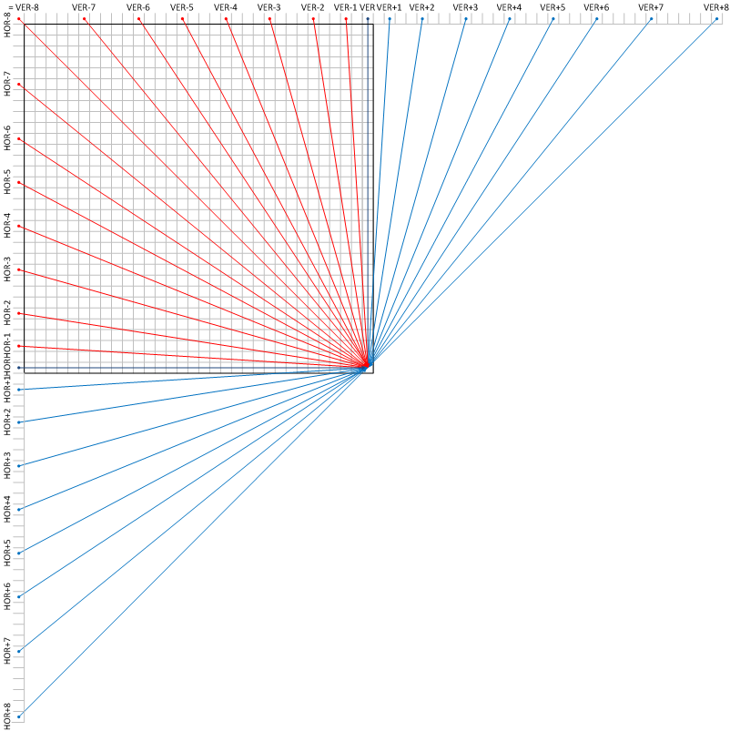 Figure 1. Available prediction directions in the unified intra prediction
Two arrays of reference samples are used in the unified intra prediction, corresponding to the row of samples lying above the current PU to be predicted, and the column of samples lying to the left of the same PU. Given a dominant prediction direction (horizontal or vertical), one of the reference arrays is defined to be the main array and the other array the side array. In the case of vertical prediction, the reference row above the PU is called the main array and the reference column to the left of the same PU is called the side array. In the case of horizontal prediction, the reference column to the left of the PU is called the main array and the reference row above the PU is called the side array.
When the intra prediction angle is positive, blue lines in Figure 1, only the samples from the main array are used for prediction. When the intra prediction angle is negative, red lines in Figure 1, a per-sample test should be performed to determine whether samples from the main or the side array should be used for prediction, as shown in Figure 2 (a). Additionally when the side array is used, the computation of the index into the side array requires a division operation. In order to remove the division operation, the lookup-table (LUT) technique is used for the negative angular prediction process in the calculation of the y-intercept in the case of vertical prediction or the x-intercept in the case of horizontal prediction. Normally, the integer and fractional parts of the intercept between are calculated using the following equations respectively:
deltaIntSide = (256*32*(l+1)/absAng)>>8
deltaFractSide = (256*32*(l+1)/absAng)%256
where absAng is the absolute value of intra prediction angle (=[ 2, 5, 9, 13, 17, 21, 26, 32]) and l is x/y pixel location for vertical/horizontal prediction. With LUT technique, the above equations can be replaced with the following equations:
deltaIntSide = (invAbsAngTable[absAngIndex]*(l+1))>>8
deltaFractSide = (invAbsAngTable[absAngIndex]*(l+1))%256
where invAbsAngTable = [4096, 1638, 910, 630, 482, 390, 315, 256]. By using LUT, there is no division operation during the computation of the index into the side array. However, there still exists the per-sample test to determine the main or the side array for prediction. To simplify this process, the main array is extended by projecting samples from the side array onto it according to the prediction direction, as shown in Figure 2 (b). During the projection, the fractional part of the intercept is omitted and the intercept is rounded to the nearest integer:
deltaInteger = (invAbsAngTable[absAngIndex]*(l+1)+128)>>8
Finally, the prediction process only uses the extended main array and the same simple linear interpolation formula to predict all samples in the PU. Figure 2 shows an example of simplified intra prediction with direction angle VER-8.
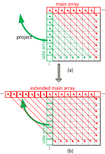
Figure 2. An example of simplified intra prediction with direction angle VER-8
When DC mode is used in the intra prediction, the mean value of samples from both top row and left column is used for the DC prediction.
Table 1 summarizes the physical and logical mode indexes used in the bitstream and prediction functions respectively. Depending on the PU size, different numbers of prediction modes are available respectively, as listed in Table 2.
Table 1. Physical and logical mode indexes used in the bitstream and prediction functions respectively
| Index | 0 | 1 | 2 | 3 | 4 | 5 | 6 | 7 | 8 | 9 | 10 | 11 |
| Physical | VER | HOR | DC | VER-8 | VER-4 | VER+4 | VER+8 | HOR-4 | HOR+4 | HOR+8 | VER-6 | VER-2 |
| Logical | DC | VER-8 | VER-7 | VER-6 | VER-5 | VER-4 | VER-3 | VER-2 | VER-1 | VER | VER+1 | VER+2 |
[......]
Permanent Link: Analysis of Coding Tools in HEVC Test Model (HM 1.0) – Intra Prediction
Analysis of Coding Tools in HEVC Test Model (HM 1.0) – Coding Structure
2010-11-30 H.265/HEVC 1 Comment Views(18,782)The HEVC test model (HM) still belongs to block-based hybrid video coding framework, except that the macroblock is extended to larger size (up to 64×64) compared with H.264/AVC. In order to facilitate syntax representation of block hierarchy, three block concepts are introduced: coding unit (CU), prediction unit (PU), and transform unit (TU). The overall coding structure is characterized by the various sizes of CU, PU and TU in a recursive manner, once the size of largest coding unit (LCU) and the hierarchical depth of CU are defined.
CU, the basic coding unit like the macroblock and sub-macroblock in H.264/AVC, can have various sizes but is restricted to be a square shape. Given the size and hierarchical depth of LCU, CU can be expressed in a recursive quadtree representation adapted to the picture. Figure 1 (b) shows maximum possible recursive CU structure in HM (LCU size = 64 and hierarchical depth = 4). In HM, the coding unit tree structure is limited from 8×8 to 64×[......]
Permanent Link: Analysis of Coding Tools in HEVC Test Model (HM 1.0) – Coding Structure
Analysis of Coding Tools in HEVC Test Model (HM 1.0) – Overview
2010-11-18 H.265/HEVC 32 Comments Views(28,400)The HEVC test model (HM) was formally established in the 3rd JCT-VC meeting in Guangzhou, China. HM only contains the minimum set of well tested tools together from a coherent design that is confirmed to show good capability, meanwhile it also follows the “one tool one functionality“ approach. It expects to closely resemble the performance of best–performing proposals, as TMuC did, and plans to contain different clusters of tools (could become a seed for profile in future) with as much commonality as possible. Currently, two configurations of typical coding tools are suggested: High Efficiency and Low Complexity, as listed in the following table.
Table 1. Structure of tools forming the high efficiency and low complexity configurations of the HM
High Efficiency
Low Complexity
Coding unit tree structure (8×8 up to 64×64 luma samples)
Prediction units
Transform unit tree structure (maximum of 3 levels)
Transform unit tree structure (maximum of 2 levels)
Transform bloc[......]
Permanent Link: Analysis of Coding Tools in HEVC Test Model (HM 1.0) – Overview
KTA employs two concatenating loop filters: the deblocking loop filter and the adaptive loop filter.
The deblocking loop filter, inherited from H.264/AVC, alleviates the blocking artifacts caused by the block-based DCT+MCP video coding framework. It uses a bank of low-pass filters, which are adaptively applied to block boundaries according to the boundary strength (BS), and provides better visual quality and improved capability to predict other pictures.
Adaptive loop filter (ALF; click here for introduction) is placed in the MCP loop after the deblocking process, and is used to restore the degraded picture (caused by compression) such that the MSE between the reconstructed and source frames is minimized. The coefficients of ALF are calculated and transmitted on a frame basis and the minimum mean squared error (MMSE) estimator is used. For each degraded frame, ALF can be applied to the entire frame or to local areas. The former is known as frame-based ALF. In the latter case, additiona[......]
Permanent Link: Two Loop Filters in KTA
Why use interpolation in video coding?
Motion-compensated prediction (MCP) is the key to the success of the modern video coding standards, as it removes the temporal redundancy in video signals and reduces the size of bitstreams significantly. With MCP, the pixels to be coded are predicted from the temporally neighboring ones, and only the prediction errors and the motion vectors (MV) are transmitted. However, due to the finite sampling rate, the actual position of the prediction in the neighboring frames may be out of the sampling grid, where the intensity is unknown, so the intensities of the positions in between the integer pixels, called sub-positions, must be interpolated and the resolution of MV is increased accordingly.
Interpolation in H.264/AVC
In H.264/AVC, for the resolution of MV is quarter-pixel, the reference frame is interpolated to be 16 times the size for MCP, 4 times both sides. As shown in Fig. 1(a), the interpolation defined in H.264 includes two stages, inter[......]
Permanent Link: Adaptive Interpolation Filter for Video Coding

